Simulating diffraction by a 2D metamaterial

Finite element simulation of the diffraction of a plane wave by a mono-periodic grating and calculation of diffraction efficiencies.

First we import the required modules and class

import numpy as np
import matplotlib.pyplot as plt
from pytheas import genmat
from pytheas import Periodic2D

Then we need to instanciate the class Periodic2D:

fem = Periodic2D()

The model consist of a single unit cell with quasi-periodic boundary conditions in the \(x\) direction enclosed with perfectly matched layers (PMLs) in the \(y\) direction to truncate the semi infinite media. From top to bottom:

• PML top

• superstrate (incident medium)

• layer 1

• design layer: this is the layer containing the periodic pattern, can be continuous or discrete

• layer 2

• substrate

• PML bottom

We define here the opto-geometric parameters:

mum = 1e-6  #: flt: the scale of the problem (here micrometers)
fem.d = 0.4 * mum  #: flt: period
fem.h_sup = 1.0 * mum  #: flt: "thickness" superstrate
fem.h_sub = 1.0 * mum  #: flt: "thickness" substrate
fem.h_layer1 = 0.1 * mum  #: flt: thickness layer 1
fem.h_layer2 = 0.1 * mum  #: flt: thickness layer 2
fem.h_des = 0.4 * mum  #: flt: thickness layer design
fem.h_pmltop = 1.0 * mum  #: flt: thickness pml top
fem.h_pmlbot = 1.0 * mum  #: flt: thickness pml bot
fem.a_pml = 1  #: flt: PMLs parameter, real part
fem.b_pml = 1  #: flt: PMLs parameter, imaginary part
fem.eps_sup = 1  #: flt: permittivity superstrate
fem.eps_sub = 3  #: flt: permittivity substrate
fem.eps_layer1 = 1  #: flt: permittivity layer 1
fem.eps_layer2 = 1  #: flt: permittivity layer 2
fem.eps_des = 1  #: flt: permittivity layer design
fem.lambda0 = 0.6 * mum  #: flt: incident wavelength
fem.theta_deg = 0.0  #: flt: incident angle
fem.pola = "TE"  #: str: polarization (TE or TM)
fem.lambda_mesh = 0.6 * mum  #: flt: incident wavelength
#: mesh parameters, correspond to a mesh size of lambda_mesh/(n*parmesh),
#: where n is the refractive index of the medium
fem.parmesh_des = 15
fem.parmesh = 13
fem.parmesh_pml = fem.parmesh * 2 / 3
fem.type_des = "elements"

We then initialize the model (copying files, etc…) and mesh the unit cell using gmsh

fem.getdp_verbose = 0
fem.gmsh_verbose = 0

fem.initialize()
mesh = fem.make_mesh()

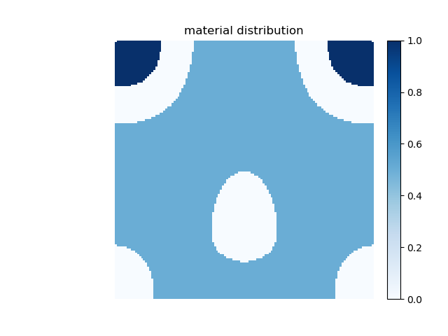
We use the genmat module to generate a material pattern

genmat.np.random.seed(100)
mat = genmat.MaterialDensity()  # instanciate
mat.n_x, mat.n_y, mat.n_z = 2 ** 7, 2 ** 7, 1  # sizes
mat.xsym = True  # symmetric with respect to x?
mat.p_seed = mat.mat_rand  # fix the pattern random seed
mat.nb_threshold = 3  # number of materials
mat._threshold_val = np.random.permutation(mat.threshold_val)
mat.pattern = mat.discrete_pattern
fig, ax = plt.subplots()
mat.plot_pattern(fig, ax)

We now assign the permittivity

fem.register_pattern(mat.pattern, mat._threshold_val)
fem.matprop_pattern = [1.4, 4 - 0.02 * 1j, 2]  # refractive index values

Now we’re ready to compute the solution:

fem.compute_solution()

Finally we compute the diffraction efficiencies, absorption and energy balance

effs_TE = fem.diffraction_efficiencies()
print("efficiencies TE", effs_TE)

Out:

efficiencies TE {'R': 0.42749531344001657, 'T': 0.45592852708133014, 'Q': 0.1177478267191832, 'B': 1.00117166724053}

It is fairly easy to switch to TM polarization:

fem.pola = "TM"
fem.compute_solution()
effs_TM = fem.diffraction_efficiencies()
print("efficiencies TM", effs_TM)

Out:

efficiencies TM {'R': 0.2052478291947634, 'T': 0.7359213200135426, 'Q': 0.05719724751542301, 'B': 0.998366396723729}

Estimated memory usage: 14 MB