Simulating diffraction by an object in 2D

Finite element simulation of the diffraction by an object illuminated by a plane wave or a line source. Calculation of scattering width and getting the field maps.

import numpy as np
import matplotlib.pyplot as plt
from pytheas import Scatt2D

plt.ion()

pi = np.pi

Then we need to instanciate the class Scatt2D:

fem = Scatt2D()
fem.rm_tmp_dir()

# We define first the opto-geometric parameters:

mum = 1  #: flt: the scale of the problem (here micrometers)
fem.lambda0 = 0.6 * mum  #: flt: incident wavelength
fem.pola = "TE"  #: str: polarization (TE or TM)
fem.theta_deg = 30.0  # 0: coming from top (y>0)
fem.hx_des = 1.0 * mum  #: flt: x thickness box
fem.hy_des = 1.0 * mum  #: flt: y thickness box
fem.h_pml = fem.lambda0  #: flt: thickness pml
fem.space2pml_L, fem.space2pml_R = fem.lambda0 * 2, fem.lambda0 * 2
fem.space2pml_T, fem.space2pml_B = fem.lambda0 * 2, fem.lambda0 * 2
fem.eps_des = 1  #: flt: permittivity design box
fem.eps_host = 1.0
fem.eps_incl = 11.0 - 1e-2 * 1j
#: mesh parameters, correspond to a mesh size of lambda_mesh/(n*parmesh),
#: where n is the refractive index of the medium
fem.lambda_mesh = 0.6 * mum  #: flt: incident wavelength
fem.parmesh_des = 10
fem.parmesh_incl = 10
fem.parmesh = 10
fem.parmesh_pml = fem.parmesh * 2 / 3

fem.Nix = 101
fem.Niy = 101

Here we define an ellipsoidal rod as the scatterer:

def ellipse(Rinclx, Rincly, rot_incl, x0, y0):
    c, s = np.cos(rot_incl), np.sin(rot_incl)
    Rot = np.array([[c, -s], [s, c]])
    nt = 360
    theta = np.linspace(-pi, pi, nt)
    x = Rinclx * np.sin(theta)
    y = Rincly * np.cos(theta)
    x, y = np.linalg.linalg.dot(Rot, np.array([x, y]))
    points = x + x0, y + y0
    return points


rod = ellipse(0.4 * mum, 0.2 * mum, 0, 0, 0)
fem.inclusion_flag = True

Initialize, build the scatterer, mesh and compute the solution:

fem.initialize()
fem.make_inclusion(rod)
fem.make_mesh()
fem.compute_solution()

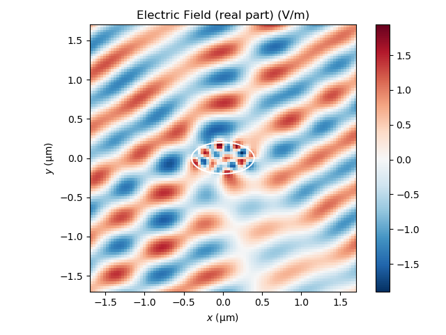
Get the electric field and plot it:

fem.postpro_fields()
u_tot = fem.get_field_map("u_tot.txt")
fig, ax = plt.subplots()
E = u_tot.real
plt.imshow(E, cmap="RdBu_r", extent=(fem.domX_L, fem.domX_R, fem.domY_B, fem.domY_T))
plt.plot(rod[0], rod[1], "w")
plt.xlabel(r"$x$ ($\rm \mu$m)")
plt.ylabel(r"$y$ ($\rm \mu$m)")
plt.title(r"Electric Field (real part) (V/m)")
plt.colorbar()
plt.tight_layout()

Do a near to far field transform and get the normalized scattering width:

ff = fem.postpro_fields_n2f()
theta = np.linspace(0, 2 * pi, 51)
scs = fem.normalized_scs(ff, theta)


fig, ax = plt.subplots()
plt.plot(theta / pi, scs, "-", c="#699545")
plt.xlabel(r"$\theta$ (rad)")
plt.ylabel(r" Normalized scattering width $\sigma/\lambda$")
ax.xaxis.set_ticks([0, 0.5, 1, 1.5, 2])
ax.xaxis.set_ticklabels(["0", "$\pi/2$", "$\pi$", "$3\pi/2$", "$2\pi$"])

scs_integ = np.trapz(scs, theta) / (2 * pi)
print("Normalized SCS", scs_integ)

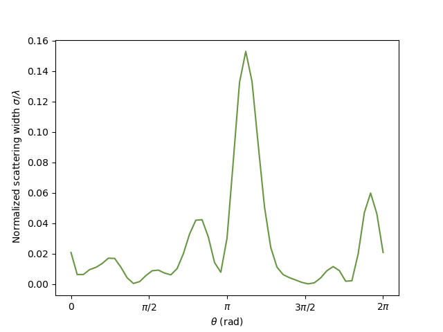
Out:

Normalized SCS 0.02572717419074843

Estimated memory usage: 16 MB